Exploring the Sanyo STK3122-III

As part of my routine management of perpetually failing appliances, I once again found myself repairing my Marantz TA170AV.  Fully suspecting the failure, and recalling that I'd mentioned it in passing once before, I figured I would approach the repair with a mind to be a bit more analytical.

This receiver came to me years ago after suffering a slow degradation of output power over the course of months.  The original owner endured the loss of one channel and then the next before gifting it to me in the traditional manner.  What better way to reduce the regret of discarding a failed investment in equipment than to let it disappear into the life of that techno-hobo friend of yours? At the time, I merely traced out the signal path and found that the STK3122 amplifier module was dead.  I replaced it with a part from a repair shop, and all was well.

The unit sat unused for nearly a decade before I dragged it out and put it into service.  After about a year or so of mild use, I began to get noise in one channel intermittently.  The noise would follow in the wake of salient bass excursions, almost like a bad volume pot, speaker switch or other poor connection.  I frustrated myself with trying to fix connections before I noticed the crossover distortion getting significantly worse.  At that point, I pulled the unit apart and checked the biasing.  Sure enough, the STK3122 was at fault again.

In the course of looking for a replacement, I began to question what I should expect.  I know that counterfeit parts exist, and I had bought the replacement from a domestic brick & mortar store, so I assumed I was in possession of two vintage modules which had failed in nominal operation.  Was there some issue with device degradation over time (metallurgical, thermomechanical, or environmental factors) which would make vintage parts inclined to be less reliable?  I bought two replacements: one was a used vintage part, and one appears to be a NOS vintage part.  Once more, I replaced the module and everything worked.

Out of curiosity, I decided to see if there was anything to be seen inside the module packaging.  The datasheet provides an internal schematic, so maybe if there were indications of a failure cause, there may be an indication of what to expect of replacement part reliability.

Note lead width and exposed substrate insulation near pin 16

Starting with the original part I'd stripped from the unit years ago, I simply used a spudger and a lacquer thinner bath to remove the nylon device cover and reveal a beautiful hybrid circuit consisting of wire-bonded bare dice and printed film resistors.  I traced out the circuit and matched it to the schematic.  It's interesting to note that this layout includes the 470 ohm resistors and pads for capacitors which would allow the external compensation networks described in the datasheet test circuit to be built internally.  I'm not sure if there was ever a family of part cousins which made use of these internal features. 

As can be seen, the bias resistors R9/R18 appear to be scratched.  On closer inspection, both resistors were open-circuit.  The top silkscreen layer over the resistive material has multiple fine cracks across it, and the conductive material is broken along two narrow cracks which show evidence of local heating.  Assuming no external circuit factors could induce this within the scope of its rated bias point, this suggests any number of things that could be at play.  Quiescent power dissipation of the package is on the order of 3W.  These things run fairly hot without a heat sink.  The observed cracks could merely be a cumulative effect of heat causing material shrinkage or degradation in a static sense.  The dynamic effect of substrate expansion could also stress these resistors.  Once cracks begin to form in the conductive printing, current crowding at the partial connection will only result in localization of resistor power dissipation and further localization of its degradation.

That's my theory anyway.  I still had a second part to dissect.  Unlike the first one which had two completely dead channels, the recent failure had one good channel and a partially failed channel.  I was hoping to be able to compare the results and see if I could determine the original value of R9 and R18.  Maybe I could even demonstrate a repair!

Note lead profiles and lack of substrate connection

After some soaking and picking and prying, I eventually got the second module apart.  Much to my surprise, it had been a counterfeit part all along.  The entire module is constructed from SMT chip resistors and SOT-23-3 parts.  Obviously, none of this will help us determine part values in a legitimate Sanyo part.  In the process of disassembly, I had noticed that the leads seemed terribly easy to bend.  When I had tested this module in a breakout board, I had similar issues. Before long, the leads started peeling off, revealing the dark copper underneath.  Most of the leads on the part show similar signs of plating/solder failure.  I am not sure that this isn't the only thing wrong with the part.  The part had demonstrated faulty output bias when in-circuit, but my tests with the part on a breakout board were varied.  If I weren't lazy and worried about abusing the receiver's PCB, I'd fix the leads and reinstall it for a test. 

More delaminated leads

I need to emphasize what pictures like this reveal.  What you're looking at are copper leads which are mechanically socketed into form-fitting solder fillets, but not necessarily electrically connected to them.  The electrical continuity between the soldered areas on the PCB and the component MCPCB may be made via intermittent semiconductive contact between copper oxides and/or intermetallics, or it may be relying on the cross sectional area of the plating alone.  Just because the leads don't wiggle around and fall off doesn't mean a reliable electrical connection exists.

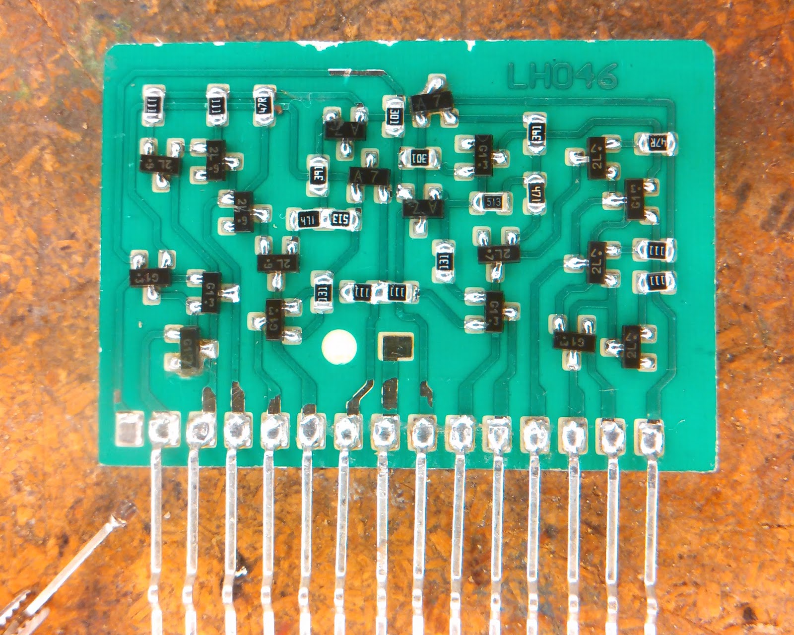
The schematic of the fake is identical to that shown in the original datasheet, though all the values are different.  All PNP transistors are MMBT5401 parts; all NPN transistors are MMBT5551 parts.  These are rather common general purpose 160v transistors.  The diode pairs are BAV99 parts.  It's noteworthy that all the parts in the counterfeit could easily be replaced.

I had to question how this handful of 0805 chips and SOT23 packages can comfortably dissipate a total of 3W.  For the moment, let's disregard the MCPCB and try a sanity check.  Assuming a limiting dissipation of 200mW per part, the module could dissipate >7W.  Of course, power isn't dissipated across all components equally.  I decided to take a look at the circuit and see if I couldn't come up with a better idea of the distribution of power in steady state.

I recreated a single channel in LTSpice and set an approximate bias point by adjustment of a dummy load with null input.  When the dummy load sets the output differential voltage to match the application schematic, the total channel dissipation matches the observed dissipation of the module. Checking the estimated component dissipation, a few things of note stick out.  Q1, Q2, and their counterparts in the other channel are operating around 80mW.  Output transistors Q7, Q8 and the counterparts are operating at around 400mW.  R9 and R18 are dissipating about 300mW each.

Keep in mind that this is just a halfass simulation with a simplified equivalent external circuit.  I fully accept that this could be inaccurate, but it falls in line with what would be expected.  Q7, Q8, and their counterparts will be the transistors with the highest dissipation.  The physical construction of the genuine hybrid part suggests this, and it's not like we can expect transistors like Q3, Q4 to contribute any significant fraction to the observed module power.

Considering Rth(j-s) values published for 0805 chips on multilayer PCB's with ground planes, 300mW on R9 and R18 doesn't seem too terrible.  The MCPCB should give these parts a lot more headroom than the worst-case values (~125mW) on a datasheet.  Then again, we have no idea what sort of value drift will occur.  The parts on the disassembled module are well within tolerance still.

Assuming it's an accurate estimation, the high dissipation on the output transistors might be of more concern.  Nominal power rating for these devices is going to be somewhere around 350mW.  This assumes minimal traces and pcb thermal conductivity.  Without a thermal resistance model for devices on a MCPCB, I simply assumed the substrate temperature is constant at 70dC.  This is higher than the observed temperature when operating without a heat sink.  Using a figure of 130K/W for Rj-c and a handwavy 10K/W for Rc-b, maximum allowable power within a 150dC junction temperature limit is somewhere around 600mW.  This is only a bit more than the highest figures for allowable package dissipation on multilayer boards.  These parts may be fine operating at 400mW, especially if the substrate has a heat sink attached. 

Of course, the thermal analysis says nothing about whether the counterfeit circuit can meet its specs in terms of noise, distortion, etc.  Although I may revisit it, I haven't bothered with much component-level testing of the fake.  I could put together a power supply and see if the quiescent dissipation follows the estimation.  I could pull the transistors in question and test them off-board to make sure they haven't been destroyed.  I may update this if I do anything more, but I'm inclined to believe that the fake was simply suffering from contact issues at the lead terminations.

While dissecting the fake doesn't help us better understand the original Sanyo part's internals, it does offer some information that will help make counterfeits identifiable.  There may be more than one breed of counterfeit out there, but I have been able to identify current Ebay listings which match this particular type. Also, this forum thread features the dissection of a fake STK3102 which matches these indicators.

• The counterfeit appears to have a facility to allow pin 8 to be bonded to the aluminum substrate, although in the example I have, there is no substrate connection at all.  Counterfeit parts may lack continuity between pin 8 and the aluminum substrate.
• The leads of the original Sanyo part are an iron alloy (magnetic), whereas the counterfeit leads are nonmagnetic. 
• The original leads also have a sheared shoulder near the package connection.  In the photos, it's easy to see that the leads are slightly wider near the bend.  The leads on the counterfeit are formed differently and have a uniform width.  
• It's also worth noting that any legitimately NOS parts will likely have heavily tarnished lead plating.  It's not a sure thing, but shiny beautiful leads are an indicator.  If you're buying a pulled part, who knows what kind of shape the leads will be in.
• The orange substrate insulation of the genuine part is visible through the lead apertures in the molded plastic shell.  This is particularly easy to see in the empty opening for pin 16.  The counterfeit part is just a MCPCB and simply shows bright green solder mask everywhere. 
• Finally, the easy way to spot some fakes is as simple as looking at the date/lot code on the front of the part.  The counterfeit part I disassembled has a code 5302.  Checking Ebay, I can find at least two "Genuine Vintage NOS" parts which have green solder mask, shiny leads, and a 5302 date code.

Ultimately, it's up to you whether the counterfeit parts are worthwhile.  Like I've commented before, I'm not against inexpensive parts in general, but if the part can't be trusted to meet its implicit specifications, its utility is severely limited.  I'm wary of the allowable power dissipation of the MCPCBA-type counterfeits, but I'm also worried about thermomechanical stresses in genuine hybrid parts.  In either case, I do suggest using a mechanically-supported heat sink on these parts. 

My take on the spare phone intercom

There are numerous tutorials online outlining methods of using landline telephones to make simple intercom systems.  While all that's really necessary to provide a talk current is a 9v battery and a resistor, ringing or otherwise signaling a call prompt to a remote station is often beyond the scope of simple designs.  About a decade ago, I put together an intercom system between the shop and the house; since I had to do some service to it recently, I figured I'll write a thing about it. 

The design is similar to the second circuit described here.  Picking up one phone causes the buzzer at the opposite station to sound.  Once both phones are off-hook, the buzzer stops.  My design changes are based around a lower voltage power supply, demonstrating that the design is certainly flexible.  The station phones can be any sort of landline phone: cordless, electronic, or just an old dumb rotary made 80 years ago.  Use twisted pair for the link cable.  Length is not likely limited in your application.  I'm using about 200 yards of cable between stations.  Any attenuation can be compensated by adjusting R3 to compensate (trim to about 25mA off-hook).

The buzzers are self-oscillating piezo buzzers.  The ones I'm using begin oscillating at about 1.5v, and as with many buzzers of this type, they can be tuned by placing a reflector of some sort at an adjustable distance in front of the aperture (I just used a tab of thin aluminum sheet).  This improves buzzer volumes at low voltages.  With higher supply voltages (24v), this may be less necessary.

Resistors R2 and R4 are used to reduce sensitivity to leakage currents or induced voltage in a long or heavily weathered link cable.  Without these bleeder resistors, a waterlogged outdoor cable or a long run of untwisted cable may result in the local station occasionally beeping weakly when both phones are on-hook.  To see why, note that the two station networks form a series voltage divider.  Any shunt conductance in the line tends to bias this voltage divider such that the local station is closer to its zener voltage than the remote station.  Since a telephone is essentially open circuit when on-hook, the divider network is very sensitive to even small shunt conductances.  Adding bleeder resistors diminishes the influence of such system defects.  For short indoor runs, they are likely unnecessary.

Switches S1 and S2 allow the station phones to function as regular landline phones.  Leaving the phone switched to the phone line does not prevent an intercom call prompt from being received.  This connection can be omitted if no landline service is desired.

Capacitors C1 and C3 allow the remote buzzer tone to be heard from the calling station. C2 is for supply bypass.  The LED can be omitted if undesired.  Use whatever power supply is handy; talk current is only 20-30 mA.  I simply used the power supply that was already in the equipment I stripped for the enclosure.

The local station in a repurposed QINGEN enclosure (and a 1941 Uniphone)

Again, this article is not unique.  Perhaps the one thing I can offer is the fact that this as-built design does function over long distances, with various phones, and for over a decade.  That's more than a 9v battery design will provide.

The problem with finding boundary chroma in CIELAB

Previously I had mentioned the use of CIELCHab and HuSL for image blending and adjustment.  Whether using LCH or a HuSL method, my approach to these operations requires the knowledge of the maximum chroma of the sRGB gamut as a function of L and H.  This isn't a simple task in CIELAB.

The extent of sRGB in CIELUV (left) and CIELAB (right)

To see why it's problematic, let's start with an existing method.  The reference implementation of HuSL uses LCHuv (CIELUV) as the parent space instead of LCHab.  The idea is the same.  For the L and H of a given pixel, we can calculate the maximum chroma for the purpose of normalization and clamping.  The approach used here is to simply calculate six boundary curves representing the intersection of the RGB gamut faces with the plane of constant L containing the given pixel.  The rest is the calculations of line-line intersections and distance minimization.

function Cout=luvboundcalc(L,H)
    % this function uses the method used by the other implementations
    % of HuSL in LUV
    Axyz=[3.240454162114103 -1.537138512797715 -0.49853140955601; ... 
        -0.96926603050518 1.876010845446694 0.041556017530349; ...
        0.055643430959114 -0.20402591351675 1.057225188223179];
    ka=903.2962962962963;
    ep=0.0088564516790356308;
    ref=[0 1];
    Cout=ones(size(L))*realmax;

    Hradians=H*pi/180;
    sinH=sin(Hradians);
    cosH=cos(Hradians);
    sub1=(L+16).^3/1560896;
    mask=(sub1>ep);
    sub2=sub1;
    sub2(~mask)=L(~mask)/ka;
    
    for r=1:3;
        row=Axyz(r,:);
        a1=row(1);
        a2=row(2);
        a3=row(3);
        top=(11120499*a1 + 11700000*a2 + 12739311*a3)*sub2;
        rbot=9608480*a3 - 1921696*a2;
        lbot=1441272*a3 - 4323816*a1;
        bot=(rbot.*sinH + lbot.*cosH).*sub2;
        
        for k=1:2;
            C=L.*(top - 11700000*ref(k))./(bot + 1921696*sinH*ref(k));
            mask=(C>0 & C<Cout);
            Cout(mask)=C(mask);
        end
    end
    Cout=min(Cout,175.2);
end

Chroma map for CIELUV at L=75 showing linear boundary curves

Although one might not suspect it at first glance, the level curves of this odd shape are indeed straight lines, and the described method works well.  We can calculate the maximal chroma for every pixel and use it to normalize or truncate an image in whole, or we can precalculate a lookup table if it makes things quicker.

The lookup table data for CIELCHuv

Discussion of HuSL elsewhere, and my own idle curiosity had to question why there was no implementation in LCHab.  Maybe I don't know enough about why it would be a dumb idea, but I like the symmetry of having both options.  Besides, if I want to do LCHab>RGB conversions, I'd want such a bounding method for the purposes of truncation anyway; again, maybe I just don't know enough.

Very quickly after trying to produce my own HuSL method in LAB, I had to wonder if the choice of LUV was in part a matter of convenience.  Unlike LUV, the level curves and meridians of the projected RGB cube are not linear.  Could we break this problem up by angle intervals and create a piecewise solution?  That's a bit problematic, as the face intersections don't lie neatly on a curve of constant H.  It would be a game of finding interval endpoints which straddle the face intersections, calculating an excess of data and then minimizing.  I start to question whether this will be costly. 

Chroma map for CIELAB at L=75, showing nonlinear boundary curves

In the process of trying to shove the LAB>RGB conversions through a solver to find a boundary curve equation, I noticed something.  At points near the yellow corner, the boundary function can't be solved as a simple function of H and L.  In simple terms, at these points there exist multiple solutions for the R=1 curve, and contrary to the required solver behavior when handling solutions from multiple curves, we want the maximum solution.

Chroma map for CIELAB at L=97.14, corresponding to the yellow corner

Detail of the above map, for H=90-120 degrees

Radials cast from the neutral axis to the primary-secondary edges intersect the R=1 face

I have yet to come up with even a conditional piecewise analytic solution. Looking around, I have not found any other approach involving an analytic solution of this bounding problem.  I ended up using a bisection solver to calculate the boundary chroma, though this approach is still very slow and a naive approach has issues converging to the apex.  Due to the undercut, convergence at the very edge would require a infinitesimally small initial step size.

I ended up performing additional calculations in the ROI near the corner, solving the R=1, G=1, and B=0 faces independently and forming a logical combination to locate the exact edge.  By this method, the numeric solver can converge to the very edge even with a large initial step size.

The lookup table data for CIELCHab, note vertical face near the problem area

function Cout=labboundcalc(L,H)
    % LUV approach won't be simple in LAB, since level curves and meridians are all nonlinear
    % furthermore, yellow corner is actually undercut and convergence at the edge 
    broadroi=H>85 & H<114 & L>85;
    pastcorner=(H-5)<L;
    ROI=(broadroi & ~pastcorner);
    
    % find boundary for entire area
    % then calculate logical combination of faces near ROI
    tic
    Cout=labsolver(L,H,1);    
    if any(ROI)
        Cbg=labsolver(L(ROI),H(ROI),2);
        Cr=labsolver(L(ROI),H(ROI),3);

        edge=(Cbg>=Cr);
        Croi=Cout(ROI);
        Croi(edge)=Cbg(edge);
        Cout(ROI)=Croi;
    end
    toc
end

function Cout=labsolver(L,H,mode)
    % adapted bisection solver for LAB
    
    % initial boundary generation for LAB
    Lc0=[0 5 33 61 67 88 98 100];
    Cc0=[30 60 135 115 95 119 97 15]+5;
    Lc=linspace(0,100);
    Cc=interp1(Lc0,Cc0,Lc);
    ind=L/100*(length(Lc)-1);
    Lp=round(ind)+1;
    
    s=size(H);
    C=Cc(Lp);
    C=reshape(C,s);
        
    % initial step sizes
    cstep=10;
    stepsize=-ones(s)*cstep;
    
    limitdelta=1E-7*prod(s);
    lastCsum=abs(sum(sum(C)));
    unmatched=true;
    out=true(s);
    first=true;
    while unmatched
        % CONVERSION MUST PASS OOG VALUES
        % bypass gamma correction for speed (results converge at the faces)
        rgb=lch2rgb(cat(3,L,C,H),'lab','nogc');

        % is point in-gamut?
        wasout=out;
        switch mode
            case 1
                out=(any(rgb<0,3) | any(rgb>1,3));
            case 2
                out=rgb(:,:,3)<0 | rgb(:,:,2)>1;
            case 3
                out=rgb(:,:,1)>1 | C<cstep;
                if first
                    fout=out;
                    first=false;
                end
        end
        neg=C<0;
        big=C>140;
        out=out & ~neg;

        change=xor(wasout,out);
        stepsize(change)=-stepsize(change)/2;
        stepsize(big)=-abs(stepsize(big));
        stepsize(neg)=abs(stepsize(neg));

        C=C+stepsize;

        Csum=abs(sum(sum(C)));
        dC=abs(Csum-lastCsum)
        lastCsum=Csum;

        if dC<limitdelta 
            unmatched=false;
        end
    end
    Cout=max(C,0);
    
    if mode==3
        Cout(fout)=150;
    end
end

This is the approach used by the function maxchroma() in my Matlab image mangling toolbox.  As mentioned, the HuSL and LCH conversion tools are based on this function.

Create a uniform colormap for plots in Matlab

This is just a quick one, and I know that there are plenty of other methods for doing this.  I figured that if I'm going to demonstrate that the symmetric normalized HuSLp and HSYp color models can be used for image editing, I might as well show other uses as well.

The symmetric models HuSLp (CIELUV and CIELAB) and HSYp (YPbPr)

Recall the nonuniformity addressed by the rotationally-symmetric normalization of HuSLp and HSYp.  While HuSL and HSY are attempts to bring the convenience of models like HSL and HSV to other, more uniform color spaces (e.g. CIELAB, CIELUV), their normalization method distorts the relationship between S and C.  A path of constant normalized saturation now has a radius dependent on hue.  To regain the uniformity of the parent space, HuSLp and HSYp are normalized to the maximal rotationally symmetric subset of the projected RGB space.  This means that HuSLp and HSYp retain visual uniformity, but at the expense of maximum chroma range.

Surfaces of maximum S: HSL (top); HuSLab, HSY (middle); HuSLpab, HSYp (bottom)

Comparing HuSL and HSY to HSL, we see the difficulty of naive color selection by simply varying hue alone.  The low resolution of these gradients makes the brightness variation much easier to notice.  The HuSLp and HSYp maps appear as a series of uniform rows.  Color selection in these maps is limited, but greatly simplified.  While care can be taken to make colormaps of higher chroma from discontinuous paths in CIELAB or YPbPr, these generic image conversion methods can be used quite easily with adequate results.

In this example, we create three colormaps corresponding to the hue angles of the primary and secondary colors.  Note the brightness variation in HSL; anyone who has spent any time making plots in Matlab has probably found themselves avoiding certain named line colors due to their poor visibility ('b' on black, 'y' on white).  While notably less saturated, the HSYp and HuSLp colormaps yield lines which are all equally visible.  Here, the HuSLp method uses CIELUV simply because the saturated corners of the RGB space are not 60 degrees apart in CIELAB. Also, take note that I'm inverting colors in the plot() call and in the imwrite() call because I'm operating with an inverted X display.

steps=6;

H=0:360/steps:(360-360/steps);
K=ones(size(H));

hslset=permute(colorspace('<hsl',cat(3,H,K,K*0.5)),[2 3 1]);
hsypset=permute(hsy2rgb(cat(3,H,K,K*0.6),'pastel'),[2 3 1]);
huslpset=permute(husl2rgb(cat(3,H,K*100,K*65),'luvp','aligned'),[2 3 1]);

lw=2;
x=0:0.01:1.4;
os=2;
d=9;
sl=1.2;
subplot_tight(1,1,1);
for n=1:1:steps;
    plot(x,     (atan(x/(n/d))-sl*x),'color',1-hslset(n,:),'linewidth',lw); hold on;
    plot(x,    -(atan(x/(n/d))-sl*x),'color',1-hslset(n,:),'linewidth',lw); hold on;
    plot(x,1*os+(atan(x/(n/d))-sl*x),'color',1-hsypset(n,:),'linewidth',lw); hold on;
    plot(x,1*os-(atan(x/(n/d))-sl*x),'color',1-hsypset(n,:),'linewidth',lw); hold on;
    plot(x,2*os+(atan(x/(n/d))-sl*x),'color',1-huslpset(n,:),'linewidth',lw); hold on;
    plot(x,2*os-(atan(x/(n/d))-sl*x),'color',1-huslpset(n,:),'linewidth',lw); hold on;
end
view(-90, 90);
set(gca,'ydir','reverse');

to=-0.45;
text(1,-to  ,'HSL','fontsize',16,'fontweight','bold');
text(1,-to+1*os,'HSYp','fontsize',16,'fontweight','bold');
text(1,-to+2*os,'HuSLpuv','fontsize',16,'fontweight','bold');

frame=getframe;
imwrite(255-frame.cdata,'blogshit/colormaps1.png','png');

Plots using colormaps generated in HSL, HSYp, HuSLp

Certainly one has to weigh uniformity against the ability to discriminate plot colors.  Strategic selection of colors based on adjacency of plot objects is often unavoidable, and at some point, one has to ask how many things should even be in a plot before a different approach to visualization is more appropriate.  Perhaps these HuSLp/HSYp palettes would be even more appropriate for creating color themes for your favorite terminal emulator.

Maybe I'll do more to extend these tools toward making discontinuous color sets at higher chroma, but I think there are plenty of people working on that already.  Then again, it's not like I'm unaccustomed to reinventing wheels.  It's not like I have anything better to do, either.

More thoughts on the 'color' blend mode

In the previous post, I discussed the 'color' image blend mode as used by GIMP and my efforts in Matlab to make a more useful variation.  To recap, methods such as HSV, HSI, and HSL in general offer poor separation of color and brightness information.  Of these methods, HSL tends to be the most useful for color adjustment and blending due to the symmetry of its saturation space, despite the fact that L is a poorer representation of image brightness than I.  Unconstrained operation in other color spaces (LAB, LUV, YPbPr) leaves us with the problem of how to deal with out-of-gamut conditions on conversion back to RGB.  Calculating boundary chroma and performing data truncation prior to RGB conversion can solve the problems caused by out-of-gamut points, resulting in good retention of background brightness.

When I had originally approached the use of LCH for image blending operations, I began by using a constrained and normalized version of LCH known originally as HuSL (now called HSLuv).  For a speed increase I also used a normalized polar version of YPbPr I refer to as HSY.  In these variations, saturation is normalized to the chroma range of the projected RGB space.  This is convenient and solves most of the same issues which a constrained LCH method solves.  It offers a few conveniences and features, but it has some weaknesses as well.  The normalization of C causes colors of constant S to no longer have a uniformity of appearance, but repeated hue adjustments do not cause chroma compression as with LCH truncation.

The projection of RGB in CIELAB and YPbPr as the extent of HuSLab and HSY

One of the drawbacks of normalizing or bounding chroma to the extent of the projected RGB space in LCH is that only a fraction of the projected RGB space lies on continuous locus of constant chroma. There exists only a small subset of the RGB space wherein color points can be subject to arbitrary hue rotation without leaving the gamut and having their chroma changed by truncation.  This maximal rotationally-symmetric boundary defines the normalizing chroma used for HuSLp, a variation of HuSL wherein the uniformity of the parent space (LAB or LUV) is retained.  As HuSLp and HSYp are subsets of the projected RGB space, they obviously cannot specify the full range of RGB colors.  Specifically, they are restricted to colors near the neutral axis, hence the suffix denoting pastel.  Compared to HuSLp, HSYp is not as uniform, but it has access to a greater fraction of the RGB space than HuSLp in either CIELAB or CIELUV modes.

Maximal biconic subsets of RGB in CIELUV, CIELAB, YPbPr

Uniformity in HuSLp (LAB): surfaces of 100% S and 50% L

Uniformity in HSYp: surfaces of 100% S and 50% Y

While this makes HuSLp and HSYp useful for color selection tasks, they are also useful for image editing so long as the chroma limiting is acceptable. Consider a color blending task with highly saturated foreground.  With its larger color range, let us compare a color blend in HSYp and LCHab.

Extreme test foreground and background

Color blends in CIELCHab and HSYp

While the limitations of HSYp are noticeable, the benefits are far more striking in this case.  The blue, red, and green stripes are moderated and the image regains its depth. 

To be realistic, this use-case is impractical but for testing.  A foreground with moderated colors would be less influenced by the limited range of HSYp.  For a sufficiently desaturated foreground, HSYp blending would produce results similar to a LCH blend, but it may still be quite a bit faster.  The major convenience of HSYp color blending is simply that the chroma is always compressed to the maximal uniform boundary.  There is no need to tweak foreground saturation to prevent uneven results.

Obviously, using stripes makes it difficult to produce a pleasing blend in any case, but that's kind of the point when testing.  In general, image editing operations need to consider content as much as method.  Blending a broad range of saturated hues with a photographic scene tends to create results which defy a viewer's expectations of reality.  Seeing a person with a purple face or a wood table lit with rainbow light doesn't make any sense to a pattern-recognition machine built on earth.

The image manipulation toolbox I've posted contains HSYp and HuSLp conversion tools, as well as support for these methods in the related image blending function (imblend) and the color adjustment function (imtweak). 

Exploring the 'color' blend mode

In my ongoing adventures in creating image manipulation tools for Matlab, I have spent quite a bit of time getting desirable behavior from blending and adjustment tools.  Although most of these problems share a common set of core difficulties, perhaps one of the more intuitive ways to explore the issue is through the common "color" layer blending mode.

In image editing tools such as GIMP and Photoshop, image layers can be combined or blended using different pixel blending modes.  While modes such as the contrast enhancing modes don't suggest their operating methods so directly, certainly the component and arithmetic modes do.  Addition and division modes suggest the underlying math.  Hue and saturation suggest the channels to be transferred between foreground and background.  The detail-oriented observer might begin to raise questions at this point.  Hue? Saturation?  In what model are we working?

What about the 'color' mode?  Mere observation suggests that it's a combination of hue and saturation information being transferred, but again, the details are critically important. Various sources online suggest that this mode performs a HS transfer in HSV... or HSB... or HSL... or HSY?  One begins to wonder if anybody knows what they're talking about.

As my experience lies with GIMP, I based my expectations on its behavior.  Certainly, I can't test my blending algo against software I don't have; however, it might be worth keeping in mind that other suites may use different approaches.  The passing impression of online resources suggests that GIMP uses HSV or HSL, Photoshop uses CIELAB, and according to simplefilter.de, PaintShopPro uses some bastard HSL/HSY swap that has people so baffled that they ask questions of forums only to get more nonsensical guidance.   Let's sort this out as best we can by simple experiment.

I assume at this point a few things about what is desired.  Forgive my loose language hereon, but in this pixel blending mode, what should be transferred is the chroma information independent of the luminosity-related information.  In other words, the hue and colorfulness should change, but not the perceived brightness.  White should remain white, black should remain black.  Acronyms make it sound like a simple task, don't they?

Let's start with HSV, HSL, and HSI.  These are polar models used to express the content of the sRGB color space.  The convenience of these familiar models is simply the manner in which their polar format allows intuitive selection and adjustment of colors.

HSV is commonly visualized as a hexagonal cone or prism defined by piecewise math.  HSI is expressed as a cylinder or cone defined by simple trigonometry.  HSL is often described as a hexagonal bicone.  What's with all the different geometry?  All we want to do is separate HS from L/V/I, right?  Feel free to look at the math, but I think it's more valuable to the novice (me) to see how the isosurfaces associated with these models are projected into the sRGB space.

Isosurfaces of Value and Intensity as projected into the RGB cube

Value, the V in HSV, is defined as the the maximum of the RGB channels.  This means that the isosurfaces of V are cube shells in RGB.  Intensity (I in HSI) is the simple average of the channels.  This translates to planar isosurfaces.  At this point, it might start to look like HSI would provide more meaningful separation of color information from brightness information.  Does it make sense that [1 1 1] and [1 0 0] have the same brightness metric as they do in HSV?  Let's try to do an HS swap in these models and see what happens.

Foreground image

Background Image

Color blend in HSV

Color blend in HSI

Well, those look terrible.  White background content is not retained, and the image brightness is severely altered.  What happens with HSL?

Color blend in HSL

Well that looks better.  In fact, that looks exactly like GIMP behaves.  Checking the source code for GIMP 2.8.14, this is exactly how GIMP behaves. Let's look for a moment at why the white content is preserved.  While I previously compared the projected brightness isosurfaces to mislead the reader as I had misled myself, the answer lies in the projection of the saturation isosurfaces.  Simply put, it is the conditional nature of the calculation of S in HSL which creates its bicone geometry and allows comparable S resolution near both the black and white corners of the RGB cube.

Saturation isosurfaces as projected into the RGB cube from HSV, HSI, HSL

So we know how GIMP does it.  What are better ways?  While HSL helps prevent the loss of white image regions, the overall brightness still suffers.  Let's start with the vague suggestion that Photoshop uses CIELAB.  At this point, I can only make educated guesses at the internals, but intuition would suggest that we might try using CIELCHab, the polar expression of CIELAB.  In naivety, I perform a CH swap to obtain the following.

Color blend in CIELCHab

Now things are actually worse.  Both black and white regions are lost.  To understand why, I put together a tool for visualizing the projection of sRGB into other color spaces such as CIELAB.

The trajectory of an out-of-gamut point in unconstrained LCHab and HuSLab

Here, we see the volume containing all RGB triplets whose values lie within standard data ranges (e.g. 0-255 for uint8).  Unlike the case with HSV, HSL, and HSI, the sRGB space is a subset of the CIELAB space.  A color point which lies outside the depicted volume would have pixel values that are either negative or larger than allowed by the datatype.  Upon conversion back to RGB, these values would be truncated to the standard range. In this manner, color points outside the cube will be mapped to points on its surface. Since the truncation occurs after conversion to RGB, the trajectory of out-of-gamut color points will be parallel to the axes of the cube.  It then stands to reason that the orientation of the neutral axis means that out-of-gamut points tend to be mapped away from the white and black corners of the cube and toward the primary-secondary edges.

If the goal remains to isolate the effects of color manipulation and image brightness, the geometry of this projection poses an issue.  To transfer the radial position of a primary or secondary corner to a pixel which is near the extent of the L axis would be to push the pixel outside the cube.  If we were to rotate the hue of a pixel which lies on a primary or secondary corner, it would again move outside the cube.  How can we manage the existence and graceful conversion of these points?   To be honest, I'm not sure I know the best methods.  All I can offer are my current approaches.

One approach would be to do data truncation prior to RGB conversion.  Of course, the maximum chroma for a given L and H is not simple to calculate, but this would keep the trajectories of out-of-gamut points in a plane of constant L.  This produces good results, but reveals an issue with working methods.

Color blend in CIELCHab

Ideally, we would try to do all our image operations in the uniform space (LAB/LUV) and only perform the conversion to RGB for final output or screen display.  At the very least, we could convert to RGB with no data truncation, allowing for negative and supramaximal pixel values to retain the information stored by OOG points.  For my efforts in creating standalone tools with RGB input and output, this best approach seems terribly impractical.  When constrained by compatibility with Matlab's image viewer and other image handling functions, we're forced to decide whether it's appropriate to lose chroma information by truncating in LCH.  Even though it causes no ill effects for a single operation, it means that successive operations will tend to compress the chroma content of the image to a small subset of the projected RGB space.

This is more of a problem for image and color adjustment than for a single channel swapping blend operation, but it's something to keep in mind.  I'll probably come back to the topic of normalized versions of LCH at a later date.

If implementing a constrained color model like this is beyond the realm of practical effort-costs, consider this simple dirty method to retain brightness in a color blend.  Simply copy the background luma, perform a HS channel swap in HSL, then re-establish the original luma using your favorite luma-chroma transformation.  This might seem like it would waste a lot of time with converting twice, but it's often the fastest method among those I've described.  The results are similar to the normalized methods, and existing conversion tools can typically be used.

Color blend in HSL with Y preservation

For an example of the methods, feel free to check out the image blending function I've posted on the Mathworks file exchange. The conversion tools for LCHab, LCHuv, HuSLab, HuSLuv, and HSY are included in the parent submission.

Remove unwanted garbage from YouTube sidebar

Nothing much to say about this one, really.  Eliminate useless clickbait bullshit from the related videos sidebar in YouTube.  Why are there 20 videos for preschool kids in the sidebar when I'm watching a video about running a lathe?  I don't want to see that shit ever again.

The way I look at it, there are at least three classes of video links that can be identified as disposable:

• Videos from certain channels
• Videos with an astronomical number of views
• Videos that are "Recommended"

I eliminate these targets with YARIP.  It might be desired to blacklist more things, but I got tired of stabbing blindly at other attempts while exploring the limited functions of XPATH 1.0.

//li[child::div/a/span[@class="stat attribution"]/span[contains(.,'Busy Beavers')]]
//li[child::div/a/span[@class="stat attribution"]/span[contains(.,'BuzzFeed')]]
//li[child::div/a/span[@class="stat attribution"]/span[contains(.,'Danger Dolan')]]
//li[child::div/a/span[@class="stat view-count" and number(translate(substring-before(.," "),',','')) > 3000000]]
//li[child::div/a/span[@class="stat view-count" and contains(., 'Recommended')]]

The particular channel names and limiting views count can be tailored for your experience and taste.